The Third Loss Rebate Theorem

By Anonymous
|
|
I thought I had completed my work on loss rebates when I published the First Loss Rebate Theorem (LRT1) in this post. Then my dog gave me a good idea on how to get a closed form for the quit-win and quit-loss points and it worked. That became the Second Loss Rebate Theorem (LRT2), given in this post. Yesterday I had a “duh” moment, and thought that I should just plug in the quit-points from LRT2 into LRT1 and solve for the maximum amount that an AP can win by exploiting a loss rebate. That ended up being a mess, but aside from algebra errors that cost me a few re-starts, it was easy. I call this result the Third Loss Rebate Theorem (LRT3).
Here is the Third Loss Rebate Theorem (click on the image to make it larger):

Here is my derivation of this result: LRT3_Proof
LRT3 is incredibly easy to use in practice. The user simply looks up the house edge and standard deviation of the game in question. For a given loss rebate amount L, the loss rebate coefficient for L can be computed with a simple spread sheet computation. LRT3 then outputs the number of units the AP will win (on average) if he follows an optimal quit-win quit-loss strategy.
Before I give some examples, I want to stress one point. We see that the maximum expected win is directly proportional to the variance (standard deviation squared) of the game, and inversely proportional to the edge. You often hear APs say that increasing variance improves the potential return by exploiting a loss rebate. This formula makes it clear. Double the standard deviation and you multiply the win-rate by 4. Double the house edge and you cut the win-rate in half.
One other quick note. A bit of scratch work will show you that maxwin > 0, no matter the values of the variables substituted into it. In other words, a corollary of LRT3 is that every unrestricted loss rebate promotion on every casino game can be beaten.
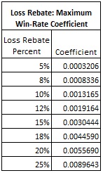
The following table gives the loss rebate coefficients for some of the most common loss rebate percentages:
Here are a couple of examples.
Example 1. Don Johnson. In his case:
Looking up 0.20 on the table above, the loss rebate coefficient is 0.0055690. It follows that the maximum expected win for Don Johnson was:
Since the “unit” for Don Johnson was $100,000, his expected win per day was $125,001.
Example 2. Single-0 Roulette, $1000 straight-up bets, loss rebate of 12%. In this case:
Looking up 0.12 on the table above, the loss rebate coefficient is 0.0019164. It follows that the maximum expected win for exploiting a 12% loss rebate by playing straight up bets on single-0 roulette is:
Since the “unit” is $1000, the maximum expected win per session is $1,208. The reader is invited to work out maxwin for single-0 roulette for the odd-even bet (σ = 0.9996, same μ and L).
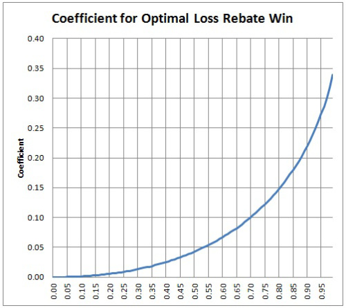
There is a feature of the loss rebate coefficients that I want to bring to light by means of an example. For a fixed game, a 10% loss rebate uses the loss rebate coefficient 0.0013165, while a 20% loss rebate uses the loss rebate coefficient 0.0055690. It follows that the maxwin available from a 20% loss rebate is (0.0055690/0.0013165) = 4.23 times that available from a 10% rebate. Offering twice the loss rebate percentage more than quadruples the vulnerability to advantage play.
Here is a plot of the loss rebate coefficient as a function of the loss rebate percentage:
As of this moment, I don’t know what else there is to do to pursue this direction of inquiry for the Loss Rebate problem. I will be taking my dog for a walk later on today, so who knows what may come next. [Note. I took the dog for a walk. No new ideas. Bad dog!]
Here is the Third Loss Rebate Theorem (click on the image to make it larger):
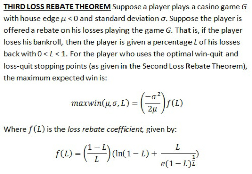
The denominator of the last term in the loss rebate coefficient kind of freaks me out. That is not "e" raised to a power. That is just "e" multiplied by that bizarre looking term (1-L)^(1/L). But this last term has its own beauty.
As the value of L goes to 0 (in the limiting case), the expression (1-L)^(1/L) converges to 1/e and f(L) goes to 0, so that the maximum expected win goes to 0. That's intuitively obvious. What is not so obvious is that as the value of L goes to 1 (in the limiting case), f(L) converges to 1/e, so that,

Here is my derivation of this result: LRT3_Proof
LRT3 is incredibly easy to use in practice. The user simply looks up the house edge and standard deviation of the game in question. For a given loss rebate amount L, the loss rebate coefficient for L can be computed with a simple spread sheet computation. LRT3 then outputs the number of units the AP will win (on average) if he follows an optimal quit-win quit-loss strategy.
Before I give some examples, I want to stress one point. We see that the maximum expected win is directly proportional to the variance (standard deviation squared) of the game, and inversely proportional to the edge. You often hear APs say that increasing variance improves the potential return by exploiting a loss rebate. This formula makes it clear. Double the standard deviation and you multiply the win-rate by 4. Double the house edge and you cut the win-rate in half.
One other quick note. A bit of scratch work will show you that maxwin > 0, no matter the values of the variables substituted into it. In other words, a corollary of LRT3 is that every unrestricted loss rebate promotion on every casino game can be beaten.
The following table gives the loss rebate coefficients for some of the most common loss rebate percentages:

Here are a couple of examples.
Example 1. Don Johnson. In his case:
- μ = -0.0029036
- σ = 1.1417
- L = 0.20
Looking up 0.20 on the table above, the loss rebate coefficient is 0.0055690. It follows that the maximum expected win for Don Johnson was:
maxwin = [(1.1417)^2/(2x0.0029036)]x(0.0055690) = 1.250013.
Since the “unit” for Don Johnson was $100,000, his expected win per day was $125,001.
Example 2. Single-0 Roulette, $1000 straight-up bets, loss rebate of 12%. In this case:
- μ = -0.0270270
- σ = 5.8378
- L = 0.12
Looking up 0.12 on the table above, the loss rebate coefficient is 0.0019164. It follows that the maximum expected win for exploiting a 12% loss rebate by playing straight up bets on single-0 roulette is:
maxwin = [(5.8378)^2/(2x0.0270270)]x(0.0019164) = 1.208264.
Since the “unit” is $1000, the maximum expected win per session is $1,208. The reader is invited to work out maxwin for single-0 roulette for the odd-even bet (σ = 0.9996, same μ and L).
There is a feature of the loss rebate coefficients that I want to bring to light by means of an example. For a fixed game, a 10% loss rebate uses the loss rebate coefficient 0.0013165, while a 20% loss rebate uses the loss rebate coefficient 0.0055690. It follows that the maxwin available from a 20% loss rebate is (0.0055690/0.0013165) = 4.23 times that available from a 10% rebate. Offering twice the loss rebate percentage more than quadruples the vulnerability to advantage play.
Here is a plot of the loss rebate coefficient as a function of the loss rebate percentage:

As of this moment, I don’t know what else there is to do to pursue this direction of inquiry for the Loss Rebate problem. I will be taking my dog for a walk later on today, so who knows what may come next. [Note. I took the dog for a walk. No new ideas. Bad dog!]


